Hello World to Quantum Computing with Qiskit
Quantum computing has long learning curve. After previous use case and concepts article, as a software developer, we also learn by doing things. Let’s start with a popular open-source quantum computing SDK: qiskit (quantum information science kit).
In traditional programming, a function is a basic building block. In quantum computing, subroutine is similarly used and to implement subroutine, you can build circuit to represent the problem you are solving. Circuit can include qubit and gates to represent computation.
Common quantum gates in qiskit in this article (more info):
single-qubit
Hadamard gate: Creates superposition
Pauli gate: Pauli-X (quantum analog of the classical NOT gate (also known as a bit-flip gate)), Pauli-Y (performs a phase flip in addition to a bit flip), Pauli-Z (applies a phase flip to the qubit (also known as a phase gate))
Two-qubit
CNOT gate: entangle and disentangle Bell states
Install qiskit and related Python packages.
pip3 install qiskit[visualization]
pip3 install jupyterlab
pip3 install matplotlib
pip3 install pylatexenc
pip3 install qiskit-aer
Follow Getting Started with Qiskit notebook for circuit basics, change following cell to use local simulator. 3 Main simulators
- Statevector gives the full quantum state as a vector.
- Unitary gives the matrix representing the combined operation of the entire circuit.
- Quasi focuses on probabilistic outcomes, especially useful when considering noisy quantum devices.
# Import Aer
# from qiskit import aer
from qiskit_aer import Aer
In addition, to display better matrix, use following method for statevector simulator
outputstate.draw(output='latex')for unitary simulator, result is not state vector but actual unitary transformation matrix (the mathematical description of the quantum circuit’s evolution)
# Convert the unitary matrix to LaTeX
unitary = result.get_unitary(circ)
Unitary matrix
Operator([[ 0.707+0.j,  0.707-0.j,  0.   +0.j,  0.   +0.j,  0.   +0.j,
            0.   +0.j,  0.   +0.j,  0.   +0.j],
          [ 0.   +0.j,  0.   +0.j,  0.   +0.j,  0.   +0.j,  0.   +0.j,
            0.   +0.j,  0.707+0.j, -0.707+0.j],
          [ 0.   +0.j,  0.   +0.j,  0.707+0.j,  0.707-0.j,  0.   +0.j,
            0.   +0.j,  0.   +0.j,  0.   +0.j],
          [ 0.   +0.j,  0.   +0.j,  0.   +0.j,  0.   +0.j,  0.707+0.j,
           -0.707+0.j,  0.   +0.j,  0.   +0.j],
          [ 0.   +0.j,  0.   +0.j,  0.   +0.j,  0.   +0.j,  0.707+0.j,
            0.707-0.j,  0.   +0.j,  0.   +0.j],
          [ 0.   +0.j,  0.   +0.j,  0.707+0.j, -0.707+0.j,  0.   +0.j,
            0.   +0.j,  0.   +0.j,  0.   +0.j],
          [ 0.   +0.j,  0.   +0.j,  0.   +0.j,  0.   +0.j,  0.   +0.j,
            0.   +0.j,  0.707+0.j,  0.707-0.j],
          [ 0.707+0.j, -0.707+0.j,  0.   +0.j,  0.   +0.j,  0.   +0.j,
            0.   +0.j,  0.   +0.j,  0.   +0.j]],
         input_dims=(2, 2, 2), output_dims=(2, 2, 2))
Which is not intuitive matrix visualization. Use array_to_latex to convert unitary matrix to Latex format like below.
from qiskit.visualization import array_to_latex
latex_matrix = array_to_latex(unitary)
from IPython.display import Latex, Markdown, HTML
display(latex_matrix)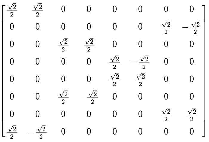
In addition, when using qasm simulator, you can get count of measurement, e.g. {‘011’: 523, ‘000’: 501}. The label is reversed, e.g. in ‘011’, the rightmost is qubit 0, middle is qubit 1, leftmost is qubit 2.
Use IBM quantum computer
pip3 install qiskit-ibm-runtimeGo to https://quantum.ibm.com/ to get your API token
from qiskit_ibm_runtime import QiskitRuntimeService
QiskitRuntimeService.save_account(channel='ibm_quantum',token='<api token>')
service = QiskitRuntimeService(channel='ibm_quantum')
backend = service.backend(name = '<QPU name>')
backend.num_qubits
# 127
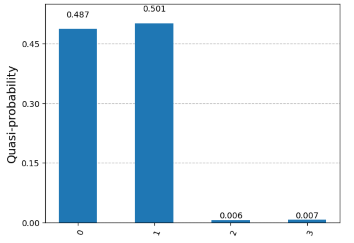
The difference between simulator and real quantum hardware is that real quantum hardware is noisy (containing errors), like below (right side is measurement on real quantum hardware)

qiskit measure: takes 2 arguments qubit, cbit). Measure a quantum bit (qubit) in the Z basis into a classical bit (cbit). It is possible to call measure with lists of qubits and cbits as a shortcut for one-to-one measurement. These two forms produce identical results:
1st
circuit = QuantumCircuit(2, 2)
circuit.measure([0,1], [0,1])
2nd
circuit = QuantumCircuit(2, 2)
circuit.measure(0, 0)
circuit.measure(1, 1)
Appendix
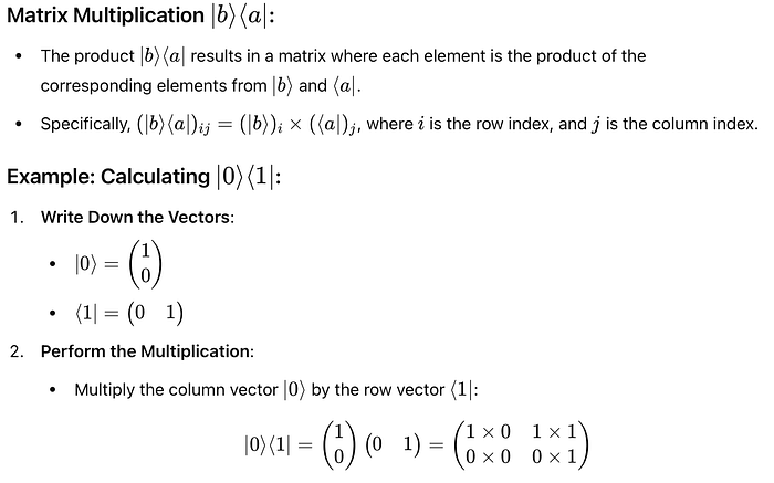
Bra Vectors (Row Vectors): ⟨a∣ represents a row vector with a 1 in the position corresponding to ‘a’ and zeros elsewhere.
For Σ={0,1}:
- ⟨0∣=(10) (since 0 is in position index 0, so index 0 is marked as 1)
- ⟨1∣=(01) (since 1is in position index 1, so index 1 is marked as 1)
Ket Vectors (Column Vectors): ∣a⟩ represents a column vector with a 1 in the position corresponding to ‘a’ and zeros elsewhere.
For Σ={0,1}:
- ∣0⟩=(10)
- ∣1⟩=(01)
absolute value ∣1+2i∣: ∣a+bi∣= sqrt(a² + b²) = sqrt(5)
Stochastic matrix represents a random process matrices, which are matrices satisfying these two properties:
- All entries are nonnegative real numbers.
- The entries in every column sum to 1.1.
Equivalently, stochastic matrices are matrices whose columns all form probability vectors.
There is also row stochastic matrix
Tensor product
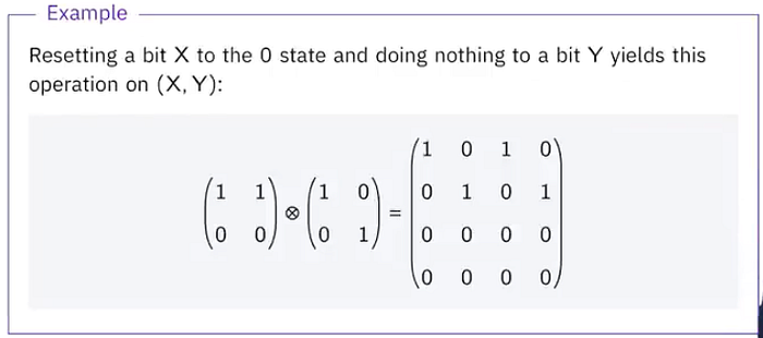
The tensor product of two or more stochastic matrices is always stochastic.
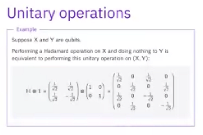
A common situation that we encounter is one in which one operation is performed on one system and nothing is done to another. In such a case, exactly the same prescription is followed, noting that doing nothing is represented by the identity matrix.
Orthogonal: Vectors are perpendicular, i.e., their dot product is zero.
Orthonormal: Vectors are orthogonal, and each vector is unit vector (has a norm (length or magnitude of a vector) of 1).
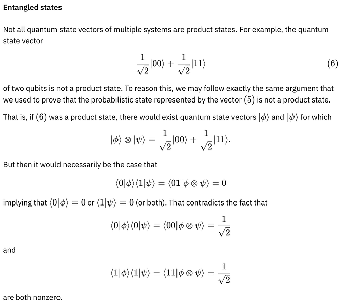
Product state vs. entangled states
In quantum mechanics it implies that the subsystem states are independent of each other. A product state of a composite quantum system consisting of subsystems AA and BB can be written as the tensor product of the individual states of each subsystem: ∣Ψ⟩=∣ϕA⟩⊗∣ϕB⟩.
Global phase: Suppose that ∣ψ⟩ and ∣ϕ⟩ are unit vectors representing quantum states of some system, and assume moreover that there exists a complex number α on the unit circle (meaning that ∣α∣=1, or alternatively α=eiθ for some real number θ) such that
∣ϕ⟩=α∣ψ⟩.
The vectors ∣ψ⟩ and ∣ϕ⟩ are then said to differ by a global phase, e.g.
∣ψ⟩=α∣0⟩+β∣1⟩
∣ψ′⟩=eiθ(α∣0⟩+β∣1⟩)
the two quantum states ∣ψ⟩ and ∣ϕ⟩ that differ by a global phase are completely indistinguishable
On the other hand, the quantum states

do not differ by a global phase. Although the only difference between the two states is that a plus sign turns into a minus sign, this is not a global phase difference, it is a relative phase (important for interference and quantum computation) difference because it does not affect every vector entry, but only a proper subset of the entries.
No-cloning theorem: unlike classical systems which is easy create an identical copy of information, it is impossible to create an exact copy of an arbitrary unknown quantum state. It’s a fundamental feature of quantum mechanics, therefore we can’t simply copy information from one qubit to another without potentially altering the original state (cannot copy without measurement and measurement alters the state).
IBM learning resources
Other learning resources


